IC-diagnostics

Martin Schobben

1 Diagnostics for Ion Count Data

The random nature of secondary ions emitted from a sample is described by Poisson statistics, and can be used to predict the precision of SIMS measurements under ideal circumstances (e.g., the predicted standard error can be deduced from the total counts of secondary ions). However, besides this fundamental source of imprecision, real SIMS measurements are additionally affected by other factors such as sample heterogeneity, instrument instability, the development and geometry of the sputter pit, and sample charging. Although some of these biases can be avoided by proper instrument tuning and sample documentation (e.g. T/SEM to characterise the textural properties of a rock sample) prior to SIMS measurement, factors such as instrument instability or sample heterogeneity can never be fully eliminated. In this vignette, diagnostic tools are showcased which can help evaluate the potential impact of such factors on the precision of ion count data.

library(point)

The following packages are used in the examples that follow.

library(purrr) # functional programming
library(dplyr) # manipulating data
library(ggplot2) # graphics

1.1 Nomenclature

• Sample: sample of the true population
• Analytical substrate: physical sample measured during SIMS analysis
• Event: single event of an ion hitting the detector
• Measurement: single count cycle \(N_i\)
• Analysis: \(n\)-series of measurements \(N_{(i)} = M_j\)
• Study: \(m\)-series of analyses \(M_{(j)}\), constituting the different spots on the analytical substrate

1.2 Basic functionality

The function diag_R() is designed to be a flexible wrapper for isotope count diagnostics. Non-isotope pairs are supported as well but the outcome is not necessarily meaningful due to variation caused by the ionization efficiency differences among elements, check the vignette IC-process for solutions. For basic functionality, diag_R() requires the following arguments: .IC, which should be a tibble containing processed ion count data (ideally, following the routine point work-flow), and arguments .ion1 and .ion2 which link to the rare isotope and common isotope, respectively (as character strings). The dots ... should be used to define a grouping variable to e.g. identify individual analysis or sets of analyses. The argument .method enables selection of diagnostic methods, which are outlined in this vignette. A range of other arguments dictate features of the returned statistics and plotting of the outcome (as a ggplot). Check ?diag_R() for all options.

In the following example the grouping structure of the data frame is defined as the file-names and block numbers, which recreates the default Cameca^TM software diagnostics.

# Use point_example() to access the examples bundled with this package 
# Carry-out the routine point work-flow
# Raw data containing 13C and 12C counts on carbonate
tb_rw <- read_IC(point_example("2018-01-19-GLENDON"), meta = TRUE)

# Processing raw ion count data
tb_pr <- cor_IC(tb_rw)

# CAMECA style diagnostics
tb_dia <- diag_R(tb_pr, "13C", "12C", file.nm, bl.nm, .method = "Cameca", 
                 .reps = 2,  .output = "diagnostic") 

The output consist of a tibble containing the single ion count statistics for each ion and the isotope ratio statistics. In addition, the specific diagnostics (selected with .method = "Cameca") is appended to the tibble. Here the procedure was repeated two times (.reps = 2) and .output set to "diagnostic" to get the augmented summary statistics of \(R\) following the Cameca^TM output.

2 Isotope ratios: A special case

Isotopes of the same element should have more-or-less the same ionization efficiency (Fitzsimons, Harte, and Clark 2000). It thus follows, that in an isotopically homogeneous analytical substrate the count rates of two isotope from the same element should be dependent on each. From this it can be deduced that large deviations in count rate ratios of an isotope system between consecutive measurements indicate a potential discrepancy (e.g., sample heterogeneity and instrument instability). This unique property enables the detection of situations in which the analysed substrate contains isotopic heterogeneity at a smaller scale than the beam size, or where machine instability causes a discrepancy in count rates between detectors.

2.1 Count block-based diagnostics (Cameca^TM)

The default method to account for such discrepancies, as incorporated in the Cameca^TM software, entails a block-wise (blocks represent sub-units of the complete analysis) check for variability. If values fall outside of a pre-defined range of variance (e.g. two standard deviations, referred to as \(\sigma\) in the Cameca^TM software), the measurement will be rejected (\(N\_rej\) in the excerpt of the Cameca output files; Fig. 2.1).

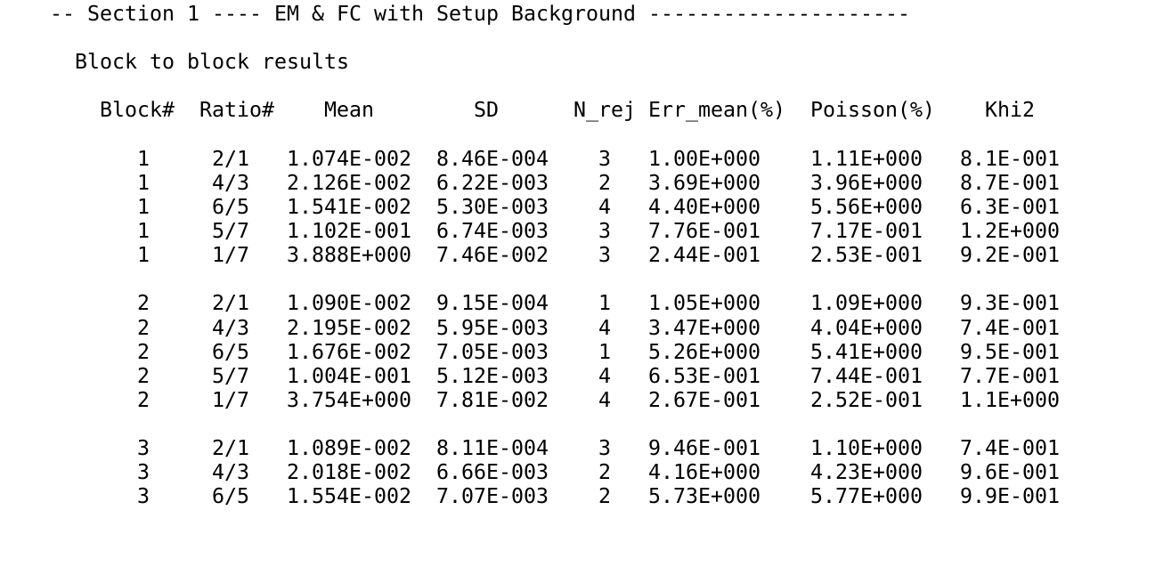
Figure 2.1: An excerpt of the Cameca stat-file for count block based 2\(\sigma\)-rejection and associated blockwise statistics

Table 2.1: Blockwise statistics for augmented dataset (replication of Fig. 2.1 with the pointpackage).

Block#	Ratio#	Mean	SD	N_rej	Err_mean (%)	Poisson (%)	Khi2
1	2/1	0.011	0.00085	3	1.00	1.11	0.81
1	5/7	0.110	0.00671	3	0.77	0.72	1.16
1	1/7	3.887	0.07454	3	0.24	0.25	0.92
2	2/1	0.011	0.00092	1	1.05	1.09	0.93
2	5/7	0.100	0.00488	5	0.63	0.75	0.70
2	1/7	3.753	0.07794	4	0.27	0.25	1.11

2.2 Regression-based diagnostics

The solution provided by the Cameca^TM software seems straightforward and effective, just compare the \(R\) values of the individual measurements of an \(n\)-series (\(N_{(i)}\)), and check whether there are significant deviations at some points during the analysis. However, the situation is more complex than that, as illustrated with the following examples.

For these examples, isotope count rates have been simulated (simu_IC provide along with the package) for three hypothetical types of materials (Fig. 2.2).

1. An “ideal” substrate with a completely homogeneous isotopic composition
   
2. A substrate with a “symmetric gradient”, which has a isotope gradient spanning the whole depth covered by the analysis
3. A substrate with an “asymmetric gradient”, which has a sudden offset in isotope composition at a specific depth

In the two simulations with a heterogeneous isotope composition the total span of isotope variability is set to 60‰. A linear trend is superimposed on the count rates of both isotope species, as this is an inherent phenomenon of SIMS analysis. This relates to changes in the ionization potential resulting from the sputter pit development and charge build-up (see vignette: IC-process). This systematic bias afflicts both isotope species to a similar degree thereby leaving \(R\) unaltered (see Fitzsimons, Harte, and Clark 2000).

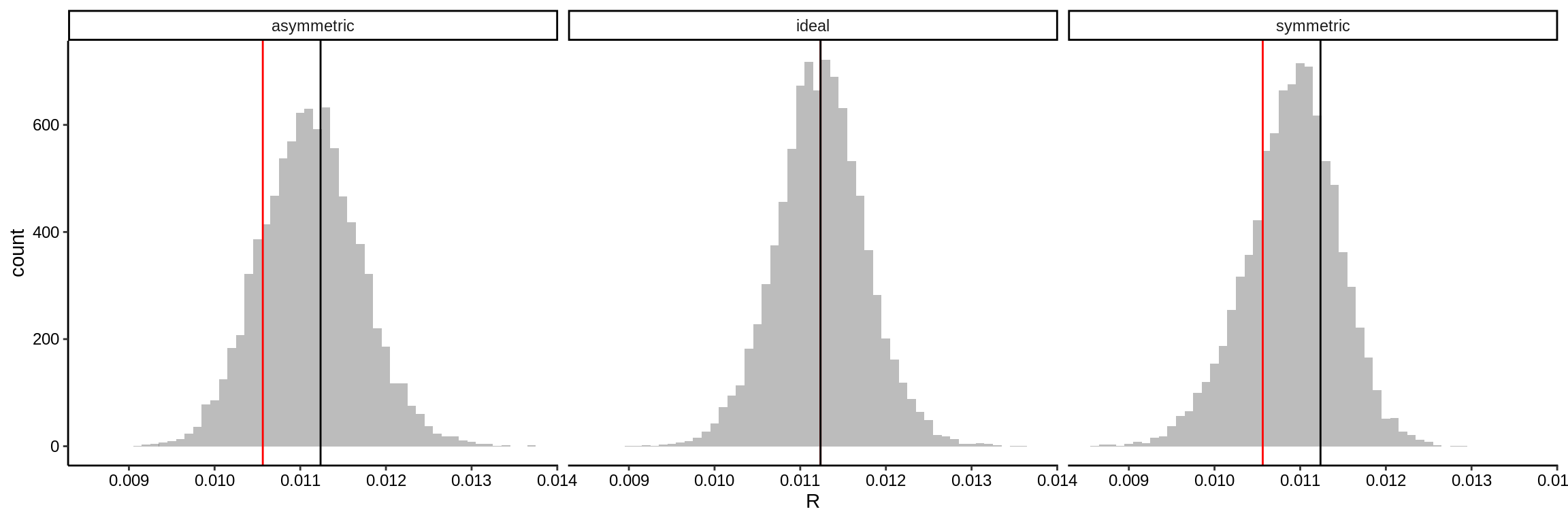
Figure 2.2: Histograms comparing input and output \(R\) values for simulations of an ideal isotopically homogenous material, a gradual gradient in \(R\) (symmetric gradient), and a sudden shift in \(R\) (asymmetric gradient).

From Figure 2.2 it is evident that the real variation in \(R\) (input R; black and red lines) are indistinguishable when viewing the derived distribution of the ion count ratios (output R; histogram). This is an effect related to the relative large random bias induced by the ionization of the substrate. So, even for these large variations in isotopic composition, it cannot be confidently said whether the measured \(R\) is representative for the analysed site, or if the underlying data structure is skewed with one, or more, isotopically distinguishable components comprising the pooled \(R\) value. This effect is, furthermore, hardly observable in the precision of the data, where the \(\epsilon_{\bar{R}}\) of the simulation referred to as “asymmetric” is 1.01, 0.97, 0.97‰, whereas the “ideal” simulation has only a marginally better precision of 0.8, 0.79, 0.8‰.

From the previous examples, it becomes apparent that heterogeneous substrates cause minimal deviation in the internal precision. Hence, a lot of hidden variation in nominal SIMS isotope analyses can go undetected. So, clearly, a different approach must be adopted to identify these isotopically highly variable substrates.

2.2.1 Linear relationship of isotope counts

In an “ideal” isotopically homogeneous substrate the count rates of two isotope from the same element should be dependent on each other (Fitzsimons, Harte, and Clark 2000). Thus, even though the ionization efficiency might vary within a single analysis, the count rate of an isotope species \(b\) can be deduced from the count rate of isotope species \(a\) through a linear combination with the isotope ratio \(R\):

\[\begin{equation} \hat{X}_i^b = \hat{R}X_i^a + \hat{e}_i \qquad \text{where} \quad e_i \sim N \left(0,\sigma^2 \right) \tag{2.1} \end{equation}\]

In this ideal linear count rate relationship, variation in \(R\) is only caused by the random nature of secondary ion generation, which follows a Poisson distribution (see vignette IC-precision). Instead of using Ordinary Least Squares (OLS) to obtain estimates for the regression coefficients, the ratio of mean ion count rates, or \(\bar{R}\), can be used as the single coefficient in this function (ratio estimation). Although the residuals (\(e_i\)) of the linear model is unobserved, it can then be approximated, as follows:

\[\begin{equation} \hat{e}_i = X_i^b - \hat{R}X_i^a \text{.} \tag{2.2} \end{equation}\]

The component \(\hat{e}_i\) gives a measure of the fit of the model (or the performance of this "ideal linear model) to the sampled data. This is known as residual analysis or regression diagnostics; see for example (Fox and Weisberg 2018). Residual analysis yield estimates about the data points that could have unduly influenced the coefficient \(\hat{R}\) of Equation (2.1). Outliers detected in linear regression can therefore be described as an observation with a response variable (isotope species; \(X_i^b\)) that is conditionally unusual when regarding the independent variable (isotope species; \(X_i^a\)).

To demonstrate this we can use again diag_R() and the simulated data according to the previous specifications (“ideal”, “symmetric”, and “asymmetric” isotope variance), and supply the nominal arguments .IC, .ion1, .ion2, ... to define again the ion count data, the isotope system to be analysed, as well as a grouping structure defining the individual analyses. We leave the .method as the default method, and plot the outcome with .plot = TRUE. The argument .label produces latex or webtex parsable labels for the data frame containing the statistics results.

tb_dia <- diag_R(simu_IC, "13C", "12C", type.nm, spot.nm, .plot = TRUE, 
                 .label = "webtex")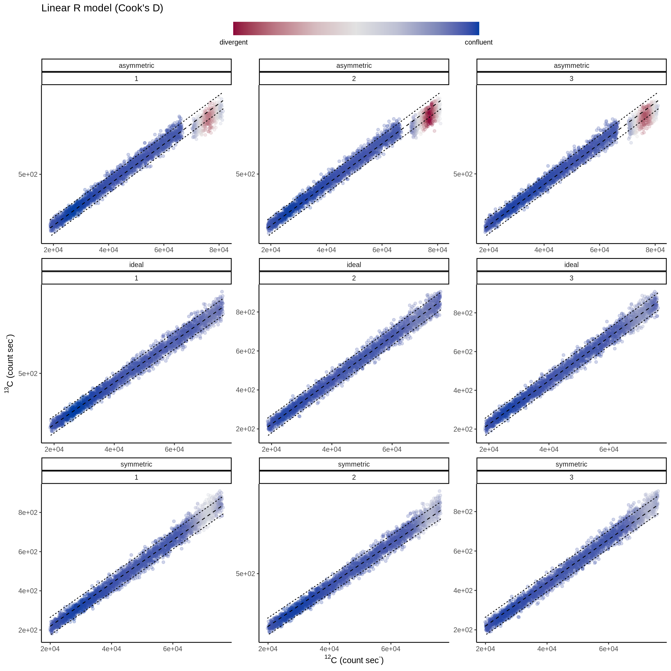

Figure 2.3: Scatter-plot of ¹³C and ¹²C count rates and the regression line following equation (2.1) and with 2 times the predicted standard deviation of the ¹³C represented as the area around the regression line demarcated with dashed lines. Here the red points identify abnormal section of the analysis with many outliers.

The simulated scenarios in Fig. 2.3 visualise the comparison of the model following Eq. (2.1) and hypothetical bivariate ¹³C-¹²C ion count rates. Anomalous sections of data-points about the model (red areas in Fig. 2.3) can already be observed in the simulations of isotopically heterogeneous substrates merely by this visualization.

For more information and a validation of this method, see the preprint:

Martin Schobben, Michiel Kienhuis, and Lubos Polerecky. 2021. New methods to detect isotopic heterogeneity with Secondary Ion Mass Spectrometry, preprint on Eartharxiv.

2.2.2 Outlier detection (Cook’s D)

The residuals will first be normalized to over come scale-dependence. This can be done by using the studentized residuals (\(\hat{e}_{i}^*\)) (see for example Fox and Weisberg 2018). A studentized residual is obtained by dividing the residual by an independent estimate of the standard deviation of the residuals. To ensure independence, the standard deviation of the residuals is calculated by leaving the residual of the \(i\)-th observation out:

\[\begin{equation} \hat{e}_i^* = \frac{\hat{e}_i}{S_{\hat{e}_{(-i)}} \sqrt{(1-h_i)}} \text{,} \tag{2.3} \end{equation}\]

where the standard error of the regression (standard deviation of the residuals) is also calculated by leaving the \(i\)-th residual out:

\[\begin{equation} S_{\hat{e}_{(-i)}} = \sqrt{\frac{1}{n-k-1} \sum_{i = 1}^{n}\hat{e}_i^2} \tag{2.4} \end{equation}\]

In Eq. (2.3) \(h_i\) represents the leverage of the independent variable (\(X^a\)), or hat-value. The hat-value measures the distance from the mean of the independent variable \(X_i^a\):

\[\begin{equation} h_i = \frac{1}{n} + \frac{ \left( X_i^a - \bar{X}_a \right)^2 }{\sum_{j=1}^n \left(X_j^a - \bar{X}_a \right)^2} \tag{2.5} \end{equation}\]

The larger the deviation \(X_i^a\) from the mean (\(\bar{X}_a\)) the more leverage the data-point has on the regression line. Given that the “ideal” simulation satisfies the conditions as initially described for the “ideal” linear model (Eq. (2.1)), the estimated \(\hat{e}\) can be used to assess deviations from this “ideal linear model”, and thereby provide a measure of how representative the \(\bar{R}\) is for the sampled spot. The goal of residual analysis would therefore be to identify the influence of the coefficient; in this case the influence on \(\bar{R}\), by determining the leverage and discrepancy (outlyingness) of variable \(X^a\), such that:

\[\begin{equation} \text{Influence} = \text{Leverage} + \text{Discrepancy} \tag{2.6} \end{equation}\]

Having already determined the outlyingness; as the studentized residuals, and the leverage; as hat-values, of the independent variable, it is possible to determine the influence of \(X^a\) have on the linear model (Eq. (2.6)). This influence can be quantified with Cook’s Distance (or Cook’s D). This formulation overcomes the effect that high leverage does not necessarily require the data-point to be influential, as Cook’s D combines the hat-values (Eq. (2.5)) with studentized residuals (Eq. (2.3)), in a new equation:

\[\begin{equation} D_i = \frac{e_{i}^{*}\phantom{}^2}{k + 1} \times \frac{h_i}{1- h_i} \tag{2.7} \end{equation}\]

Here, the \(k\) stands for the number of coefficients in the regression model. To quantify whether \(D_i\) is substantially larger then the rest of the sample’s \(D\) a cut-off value can be defined as follows.

\[\begin{equation} D_c =4/ (n-k-1) \tag{2.8} \end{equation}\]

These calculations are internally performed by a consecutive call to base lm() and broom::augment() (Robinson, Hayes, and Couch 2022).

2.2.3 Detecting intra-analysis isotope varaibility with significant outliers

The effectiveness of recognising and differentiating the “ideal” substrate from compromised measurements detected with e.g. Cook’s D (or other outlier detection methods) can now be calculated by assessing the impact on the averaged \(R\) value. This can be achieved by applying a joint model coefficient hypothesis test (or Fisher test), where the diag_R() function is designed to measure this deviation from the ideal “homogeneous” model (Eq. (2.1) by default.

\[\begin{equation} F_{(q-p),(n-q)} = \frac{ (RSS_{\theta_{0}}-RSS_{\theta_{1}}) / (q-p) }{RSS_{\theta_{1}} / (n-q)} \tag{2.9} \end{equation}\]

The default settings of the diag_R() function produces the following outcome.

execution	type.nm	spot.nm	ratio.nm	\(\bar{R}\)	\(F_{R}\)	\(p_{R}\)
1	asymmetric	1	13C/12C	0.0111	63	0.00
1	asymmetric	2	13C/12C	0.0111	75	0.00
1	asymmetric	3	13C/12C	0.0111	72	0.00
1	ideal	1	13C/12C	0.0112	0	0.85
1	ideal	2	13C/12C	0.0112	0	0.88
1	ideal	3	13C/12C	0.0112	2	0.16
1	symmetric	1	13C/12C	0.0110	105	0.00
1	symmetric	2	13C/12C	0.0110	127	0.00
1	symmetric	3	13C/12C	0.0110	122	0.00

Here, the \(F_{R}\) refers to the Fisher test statistic and the associated significance value as \(p_{R}\).

Sensitivity runs (outlined in Schobben, Kienhuis and Polerecky, in prep) show that the Cook’s D outlier detection method performs best when compared to other methods. Hence, problematic analyses with possible intra-analysis isotope variability can be detected, even if this is not obvious from the descriptive and predictive statistics alone.

2.3 Inter-analysis isotope variability

The diag_R() is designed in resemblance to the stat_R() function, and thus also includes an option to check the external structure of the the \(m\)-series of analyses usually comprised in a SIMS-based study (i.e. severeal sputter pits). For this purpose, again an .nest argument is included to define the grouping structure of individual analysis. In the simulated example this could refer to the different scenarios of isotopic variations (“ideal”, “symmetric”, and “asymmetric” isotope variance). And, this then provides a test for inter-analysis isotope variability (among the sputter pits), and can be conducted as follows.

tb_ext <- diag_R(simu_IC, "13C", "12C", type.nm, spot.nm, .nest = type.nm, 
                 .label = "webtex")

execution	type.nm	spot.nm	ratio.nm	\(\bar{R}\)	\(F_{R}\)	\(p_{R}\)	\(\hat{\bar{R}}\)	\(\hat{\epsilon}_{\bar{R}}\) (‰)	\(\Delta AIC_{\bar{R}}\)	\(p_{\bar{R}}\)
1	asymmetric	1	13C/12C	0.0111	63	0.00	0.0111	14.7	606	0
1	asymmetric	2	13C/12C	0.0111	75	0.00	0.0111	14.3	592	0
1	asymmetric	3	13C/12C	0.0111	72	0.00	0.0111	14.3	595	0
1	ideal	1	13C/12C	0.0112	0	0.85	0.0111	14.7	606	0
1	ideal	2	13C/12C	0.0112	0	0.88	0.0111	14.3	592	0
1	ideal	3	13C/12C	0.0112	2	0.16	0.0111	14.3	595	0
1	symmetric	1	13C/12C	0.0110	105	0.00	0.0111	14.7	606	0
1	symmetric	2	13C/12C	0.0110	127	0.00	0.0111	14.3	592	0
1	symmetric	3	13C/12C	0.0110	122	0.00	0.0111	14.3	595	0

This test provides and approximation of the “grand mean” (\(\bar{\bar{R}} = \frac{1}{m}\sum_{j =1}^{m}\bar{R}_j\)) of the study \(\hat{\bar{R}}\). If the substrate would be isotopically homogeneous across its surface, then each analysis would approach \(\bar{\bar{R}}\). This can again be described by the ideal “homogeneous” model of Equation (2.1), where the \(m\)-series is viewed as one long analysis of \(n\)-measurements (\(m\sum_{i=1}^{n}X_{i}^{a \mid b}\)). Introduction of a nominal factorial that interacts with \(\hat{R}\) can therefore again be used, but now to account for inter-analysis isotope variability. The major difference of this approach is that in this case the levels are encoded to represent the \(j\)-th analysis of the \(m\)-series of analyses. Encoding of this nominal variable can in theory constitute as many analyses as needed, potentially creating excessive parameters when considered as a fix component. This grouping structure, that is of no particular interest, is therefore instead represented as a random effect. This introduces a second level in Equation (2.1), where each group (\(j\)-th analysis) can assume a different \(\hat{R}\), that is, different \(\bar{R}\) may exist among the various analysis.

\[\begin{equation} \text{level 1:} \quad \hat{X}_{ij}^b = \hat{R}_{j}X_{ij}^a + e_{ij} \qquad \text{where} \quad e_{ij} \sim N(0,\sigma^2) \end{equation}\]

\[\begin{equation} \text{level 2:} \quad \hat{R}_{j} = \hat{\bar{R}} + u_{j} \qquad \text{where} \quad u_{j} \sim N(0, t^2) \tag{2.10} \end{equation}\]

Coefficients for this mixed linear model are obtained by Restricted Maximum Likelihood (REML) optimization using the lme() function of the nlme package (Pinheiro, Bates, and R Core Team 2022). The ratio of the obtained log-likelihood (i.e., maximized likelihood functions) for the restricted model and the unrestricted model, or likelihood-ratio test (LR), can the be applied to deduce the significance of including a random component in Equation (2.1). Here, a larger difference in the AIC (\(\Delta AIC_{\bar{R}}\)) and thus lower \(p_{\bar{R}}\) indicates that the null model of no inter-analysis isotope variability becomes less appropriate.

References

Fitzsimons, I. C. W., B. Harte, and R. M. Clark. 2000. “SIMS stable isotope measurement: counting statistics and analytical precision.” Mineralogical Magazine 64 (01): 59–83. https://doi.org/10.1180/002646100549139.

Fox, John, and Sanford Weisberg. 2018. An R companion to applied regression. Sage publications.

Pinheiro, José, Douglas Bates, and R Core Team. 2022. Nlme: Linear and Nonlinear Mixed Effects Models. https://svn.r-project.org/R-packages/trunk/nlme/.

Robinson, David, Alex Hayes, and Simon Couch. 2022. Broom: Convert Statistical Objects into Tidy Tibbles. https://CRAN.R-project.org/package=broom.