Diagnostics isotope count data — diag

diag_R wrapper function for diagnostics on isotope count data

Usage

diag_R(
  .IC,
  .ion1,
  .ion2,
  ...,
  .nest = NULL,
  .method = "CooksD",
  .reps = 1,
  .X = NULL,
  .N = NULL,
  .species = NULL,
  .t = NULL,
  .output = "inference",
  .label = "none",
  .meta = FALSE,
  .alpha_level = 0.05,
  .hyp = "none",
  .plot = FALSE,
  .plot_type = "static",
  .plot_stat = NULL,
  .plot_iso = FALSE,
  .plot_outlier_labs = c("divergent", "confluent"),
  .mc_cores = 1
)

Arguments

.IC: A tibble containing processed ion count data.
.ion1: A character string constituting the rare isotope ("13C").
.ion2: A character string constituting the common isotope ("12C").
...: Variables for grouping.
.nest: A variable hat identifies a series of analyses to calculate the significance of inter-isotope variability.
.method: Character string for the method for diagnostics (default = "CooksD", see details).
.reps: Numeric setting the number of repeated iterations of outlier detection (default = 1).
.X: A variable constituting the ion count rate (defaults to variables generated with read_IC())
.N: A variable constituting the ion counts (defaults to variables generated with read_IC().).
.species: A variable constituting the species analysed (defaults to variables generated with read_IC()).
.t: A variable constituting the time of the analyses (defaults to variables generated with read_IC()).
.output: Can be set to "complete" which returns stat_R() and stat_X() statistics, diagnostics, and inference test results following the selected method (see above argument .method); "augmented" for the augmented IC data after diagnostics; "diagnostic" returns stat_R() and stat_X() statistics and outlier detection; "outlier" for outlier detection; "inference" for only inference test statistics results (default = "inference").
.label: For printing nice latex labels use "latex" (default = NULL).
.meta: Logical whether to preserve the metadata as an attribute (defaults to TRUE).
.alpha_level: Significance level of hypothesis test.
.hyp: Hypothesis test appropriate for the selected method (default = "none").
.plot: Logical indicating whether plot is generated.
.plot_type: Character string determining whether the returned plot is "static" ggplot2::ggplot2()(currently only supported option).
.plot_stat: Adds a statistic label to the plot (e.g. . "M"), see point::nm_stat_R for the full selection of statistics available.
.plot_iso: A character string (e.g. "VPDB") for the delta conversion of R (see ?calib_R() for options).
.plot_outlier_labs: A character vector of length two for the colourbar text for outliers (default = c("divergent", "confluent")).
.mc_cores: Number of workers for parallel execution (Does not work on Windows).

Value

A ggplot2::ggplot() is returned (if .plot = TRUE) along with a tibble::tibble() which can contain statistics diagnostics, hypothesis test results associated with the chosen method and depending on the argument .output.

Details

The diag_R function performs an internal call to stat_R to perform diagnostics on the influence of individual measurements on the block-wise or global (i.e., a complete analysis) statistics. It identifies potentially influential measurements that indicate heterogeneity in the analytical substrate or measurement. See vignette("IC-diagnostics", package = "point") for more information on how to use the function, and possible methods for outlier detection. Options are "CooksD" (default), "Cameca", "Rm", "norm_E", "CV", "IR", and "QQ", see the vignette("IC-diagnostics", package = "point") for examples and point::names_plot. The argument .output can be used to toggle between "complete"; returning stat_R() and stat_X() statistics, diagnostics, and inference test results, "augmented"; returning the augmented IC after removing outliers, "diagnostic"; for only outlier detection results; "diagnostic"; for statistics and outlier detection, or "inference"; returns only inference test statistics results (default = inference).

Examples

# Modelled ion count dataset
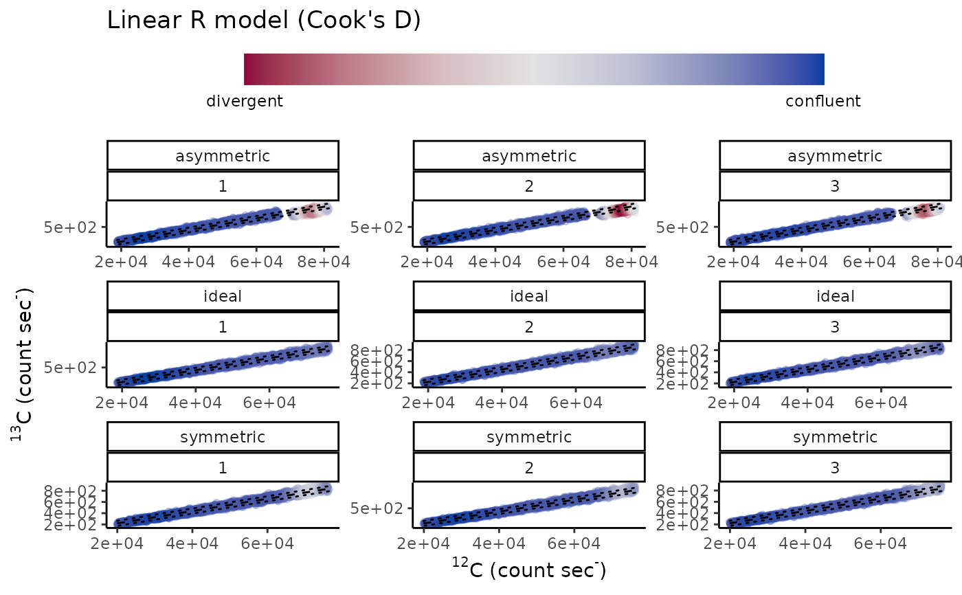
# Cook's D style diagnostic-augmentation of ion count data for
# isotope ratios
diag_R(simu_IC, "13C", "12C", type.nm, spot.nm, .plot = TRUE)

#> # A tibble: 9 × 7
#>   execution type.nm    spot.nm ratio.nm M_R_Xt.pr F_R_Xt.pr p_R_Xt.pr
#>       <dbl> <chr>        <int> <chr>        <dbl>     <dbl>     <dbl>
#> 1         1 asymmetric       1 13C/12C     0.0111    63.2    1.28e-39
#> 2         1 asymmetric       2 13C/12C     0.0111    74.9    1.09e-46
#> 3         1 asymmetric       3 13C/12C     0.0111    71.9    6.70e-45
#> 4         1 ideal            1 13C/12C     0.0112     0.267  8.49e- 1
#> 5         1 ideal            2 13C/12C     0.0112     0.219  8.83e- 1
#> 6         1 ideal            3 13C/12C     0.0112     1.73   1.59e- 1
#> 7         1 symmetric        1 13C/12C     0.0110   105.     2.00e-64
#> 8         1 symmetric        2 13C/12C     0.0110   127.     2.81e-77
#> 9         1 symmetric        3 13C/12C     0.0110   122.     1.42e-74