IC-read

1 Reading Raw Ion Count Data

The read functions are currently only supported for data generated by a Cameca NanoSIMS 50L. Raw ion count data and accompanying metadata is extracted and collated into a single tibble from text files with the extensions .is_txt, .chk_is and .stat, respectively. These files can usually be found in a single directory, which often constitute the analysis on a series of spots.

2 Nomenclature

Sample: sample of the true population
Analytical substrate: physical sample measured during SIMS analysis
Event: single event of an ion hitting the detector
Measurement: single count cycle $N_i$
Analysis: $n$-series of measurements $N_{(i)} = M_j$
Study: $m$-series of analyses $M_{(j)}$, constituting the different spots on the analytical substrate

library(point) # load package

The following packages are used in the examples that follow.

library(dplyr) # manipulating data
library(ggplot2) # plot
library(polyaAeppli) # Polya-Aeppli distribution
library(purrr) # functional programming
library(tidyr) # tidyr data

3 Example dataset

One example dataset is bundled with this package: 2018-01-19-GLENDON.

The dataset is generated with the Cameca NanoSIMS 50L at the Department of Earth Sciences at Utrecht University. The suffix GLENDON stands for glendonite an authigenic calcium carbonate seafloor precipitate. The excerpt included here contains an in-house reference (a belemnite rostra) which was used to check repeatability/external reproducibility. Ion detection for 7 individual species was performed solely with electron multipliers (EM) with the main purpose of producing stable carbon isotope ratios (¹³C/¹²C).

The example directories can be accessed with the function point_example().

# Use point_example() to access the examples bundled with this package 
# If path is 'NULL', the example directories will be listed
point_example()
#> [1] "2018-01-19-GLENDON"
# Accessing the example directory 2018-01-19-GLENDON
point_example("2018-01-19-GLENDON")
#> [1] "/home/runner/.cache/R/renv/library/point-ffcd8613/R-4.2/x86_64-pc-linux-gnu/point/extdata/2018-01-19-GLENDON"

4 Extracting raw ion count data and associated metadata

The function read_IC() takes a character string indicating the directory file name. It further enables selecting the extraction of associated metadata by setting the argument meta = TRUE (default), and this metadata can be include as an attribute with argument hide = TRUE (default) or as additional columns hide = FALSE. This has the added bonus that it provides consistency checks between metadata that generate easily interpretable warnings.

(tb_rw <- read_IC(point_example("2018-01-19-GLENDON"), meta = TRUE))
#> Registered S3 methods overwritten by 'readr':
#>   method                    from 
#>   as.data.frame.spec_tbl_df vroom
#>   as_tibble.spec_tbl_df     vroom
#>   format.col_spec           vroom
#>   print.col_spec            vroom
#>   print.collector           vroom
#>   print.date_names          vroom
#>   print.locale              vroom
#>   str.col_spec              vroom
#> # A tibble: 81,900 × 7
#>    file.nm                 t.nm  N.rw species.nm sample.nm         n.rw bl.nm
#>    <chr>                  <dbl> <dbl> <chr>      <chr>            <dbl> <int>
#>  1 2018-01-19-GLENDON_1_1  0.54 12040 12C        Belemnite,Indium  3900     1
#>  2 2018-01-19-GLENDON_1_1  1.08 11950 12C        Belemnite,Indium  3900     1
#>  3 2018-01-19-GLENDON_1_1  1.62 12100 12C        Belemnite,Indium  3900     1
#>  4 2018-01-19-GLENDON_1_1  2.16 11946 12C        Belemnite,Indium  3900     1
#>  5 2018-01-19-GLENDON_1_1  2.7  12178 12C        Belemnite,Indium  3900     1
#>  6 2018-01-19-GLENDON_1_1  3.24 12114 12C        Belemnite,Indium  3900     1
#>  7 2018-01-19-GLENDON_1_1  3.78 12147 12C        Belemnite,Indium  3900     1
#>  8 2018-01-19-GLENDON_1_1  4.32 12092 12C        Belemnite,Indium  3900     1
#>  9 2018-01-19-GLENDON_1_1  4.86 12024 12C        Belemnite,Indium  3900     1
#> 10 2018-01-19-GLENDON_1_1  5.4  12045 12C        Belemnite,Indium  3900     1
#> # … with 81,890 more rows

This generates a tibble which includes;

file.nm: file name
t.nm: time increments of the measurements $t_i$
N.rw: the individual measurement counts $N_i$
species.nm: chemical species name
sample.nm: physical sample name
n.rw: the total number of measurements $n$
bl.nm: count block identifier

Warnings signals are used to inform to inform that e.g. some metadata files have no associated data files with ion counts. These files are omitted with this argument combination call to read_IC().

The data is complemented with metadata of the associated analysis.

attr(tb_rw, "metadata")
#> # A tibble: 81,900 × 38
#>    file.nm       t.nm species.nm sample.nm bl.nm num.mt bfield.mt rad.mt mass.mt
#>    <chr>        <dbl> <chr>      <chr>     <int>  <dbl> <chr>     <chr>  <chr>  
#>  1 2018-01-19-…  0.54 12C        Belemnit…     1      1 1435.746  310.6… 12.000…
#>  2 2018-01-19-…  1.08 12C        Belemnit…     1      1 1435.746  310.6… 12.000…
#>  3 2018-01-19-…  1.62 12C        Belemnit…     1      1 1435.746  310.6… 12.000…
#>  4 2018-01-19-…  2.16 12C        Belemnit…     1      1 1435.746  310.6… 12.000…
#>  5 2018-01-19-…  2.7  12C        Belemnit…     1      1 1435.746  310.6… 12.000…
#>  6 2018-01-19-…  3.24 12C        Belemnit…     1      1 1435.746  310.6… 12.000…
#>  7 2018-01-19-…  3.78 12C        Belemnit…     1      1 1435.746  310.6… 12.000…
#>  8 2018-01-19-…  4.32 12C        Belemnit…     1      1 1435.746  310.6… 12.000…
#>  9 2018-01-19-…  4.86 12C        Belemnit…     1      1 1435.746  310.6… 12.000…
#> 10 2018-01-19-…  5.4  12C        Belemnit…     1      1 1435.746  310.6… 12.000…
#> # … with 81,890 more rows, and 29 more variables: tc.mt <dbl>, coord.mt <chr>,
#> #   file_raw.mt <chr>, bl_num.mt <chr>, meas_bl.mt <chr>, rejection.mt <chr>,
#> #   slit.mt <chr>, lens.mt <chr>, presput.mt <chr>, rast_com.mt <chr>,
#> #   frame.mt <chr>, blank_rast.mt <chr>, raster.mt <chr>, tune.mt <chr>,
#> #   reg_mode.mt <chr>, chk_frm.mt <chr>, sec_ion_cent.mt <chr>,
#> #   frame_sec_ion_cent.mt <chr>, width_hor.mt <chr>, width_ver.mt <chr>,
#> #   E0S_cent.mt <chr>, width_V.mt <chr>, E0P_off.mt <chr>, …

num.mt: measurement order in case of multiple chemical species
mass.mt: mass measured
det.mt: number of the detector trolley
tc.mt: measurement time of a measurement blanked in seconds
rad.mt: radius of the mass spectrometer
sample.nm: the assigned sample name
data: date of the analysis
presput.mt: time allocated for presputtering of the analytical substrate in seconds
bl_num.mt: block number
meas_bl.mt: number of measurements per block
width_hor.mt: horizontal Secondary Ion Beam Centering in Volts
width_ver.mt: vertical Secondary Ion Beam Centering in Volts
prim_cur_start.mt: Primary Ion Beam current in pico Ampere at the beginning of the analysis
prim_cur_after.mt: Primary Ion Beam current in pico Ampere at the end of the analysis
rast_com.mt: raster dimensions in micrometer
blank_rast.mt: percentage of blanked raster
det_type.mt: the type of ion counting devise; Electron Multiplier (EM) or Faraday Cup (FC)

In the case of EM usage for ion counting the metadate is complemented with;

mean_PHD.mt: the mean pulse height amplitude in Volts to approximate the peak height distribution (PHD)
SD_PHD.mt: the standard deviation of pulse height amplitude in Volts to approximate the PHD
EMHV.mt: EM High Voltage

In the case of FC usage for ion counting the metadate is complemented with;

FC_start.mt: FC background count before data acquisition
FC_after.mt: FC background count after data acquisition

5 Extracting metadata for machine performance assessment

Alternatively, one can also only extract the metadata of an analysis to, e.g., assess machine performance over a sequence of analyses. For example, one can assess the Peak Height Distribution (PHD) over a series of analyses.

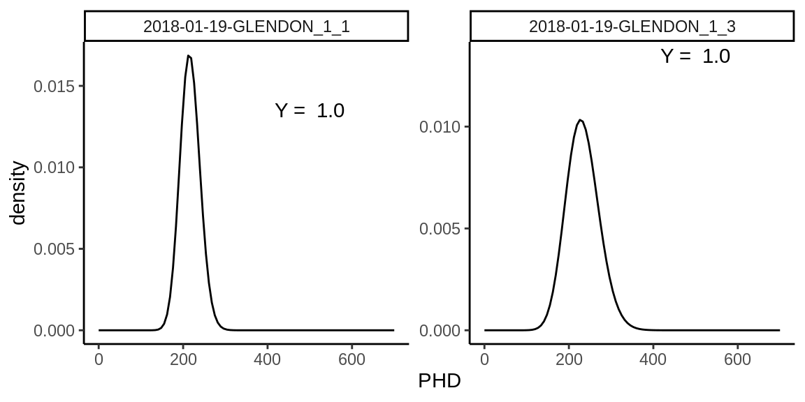
$The PHD with normalised units on the Y-axis approximated with the Polya-Aeppli density probability function with parameter $\lambda$ and $p$ for the location and shape of the curve. These parameters can be calculated using the metadata variables mean_PHD (mean) and SD_PHD (variance), which are compiled by the read_meta function.$

Figure 5.1: The PHD with normalised units on the Y-axis approximated with the Polya-Aeppli density probability function with parameter $\lambda$ and $p$ for the location and shape of the curve. These parameters can be calculated using the metadata variables mean_PHD (mean) and SD_PHD (variance), which are compiled by the read_meta function.

The compounded Polya-Aeppli density probability function can approximate the peak height distribution (Dietz 1970; Dietz and Hanrahan 1978). The package pPolyaAeppli (Burden 2014) together with the discriminator threshold value (usually 50 V) enables calculating the EM Yield ($Y$) (Fig. 5.1). More on this topic can be found in the vignette IC-process.

References

Burden, Conrad J. 2014. “An R Implementation of the Polya-Aeppli Distribution.” http://arxiv.org/abs/1406.2780.

Dietz, L. A. 1970. “General method for computing the statistics of charge amplification in particle and photon detectors used for pulse counting.” International Journal of Mass Spectrometry and Ion Physics 5 (1-2): 11–19. https://doi.org/10.1016/0020-7381(70)87002-4.