IC-process

1 Accuracy of Ion Count Data

Systematic bias can be introduced by the way secondary ions are generated from primary Cs⁺ and O^- bombardment on the analytical substrate as well as the ion-to-electron conversion efficiency in the detection systems. Commonly used detection system are electron multipliers (EM) for low secondary ion currents and Faraday cups (FC) for high secondary ion currents.

1.1 Nomenclature

Sample: sample of the true population
Analytical substrate: physical sample measured during SIMS analysis
Event: single event of an ion hitting the detector
Measurement: single count cycle $N_i$
Analysis: $n$-series of measurements $N_{(i)} = M_j$
Study: $m$-series of analyses $M_{(j)}$, constituting the different spots on the analytical substrate

library(point) # load package

The following packages are used in the examples that follow.

library(dplyr) # manipulating data
library(ggplot2) # manipulating strings
library(polyaAeppli) # Polya-Aeppli distribution
library(tibble) # tibble dataframe

1.2 Systematic bias by ion detection devices

1.2.1 Analytical bias introduced by electron multipliers

The EM gain is a measure of the electron output current relative to the ion input and the amplification after ion-to-electron conversion. In this process an incident secondary ion triggers the generation of an electron at the first dynode (conversion dynode) of the EM channel; in turn, the resultant secondary electron strikes a consecutive dynode thereby amplifying the signal, where the latter process of secondary electron amplification is repeated multiple times (for the Cameca NanoSIMS 50L this generally results in a gain of $10^8$ electrons).

Figure 1.1: Graphic representation of the EM ion detection device

After this phase of successive cascading charge amplification, the signal is converted to voltage (the EM high voltage, or EMHV; see Fig. 1.1), where the voltage is proportional to the EM gain. This last conversion depends on the age of the EM and the EMHV is usually increased with successive age to preserve ion-to-electron efficiency at a suitable sensitivity.

1.2.1.1 Electron Multiplier Yield

The amplitude of EM secondary electron output to EMHV conversion follows the so-called Peak Height Distribution (PHD). In tuning the EM detection system, the EM secondary electron output to EMHV conversion is optimized so that the probability of an electron output to have a certain EMHV is higher than a pre-defined threshold. This discriminator threshold is set to filter-out the background noise (typically 5$\,$ct$\,$s^-). However the discriminator threshold will inevitably also cut-off part of the genuine EM secondary electron output (Slodzian et al. 2001).

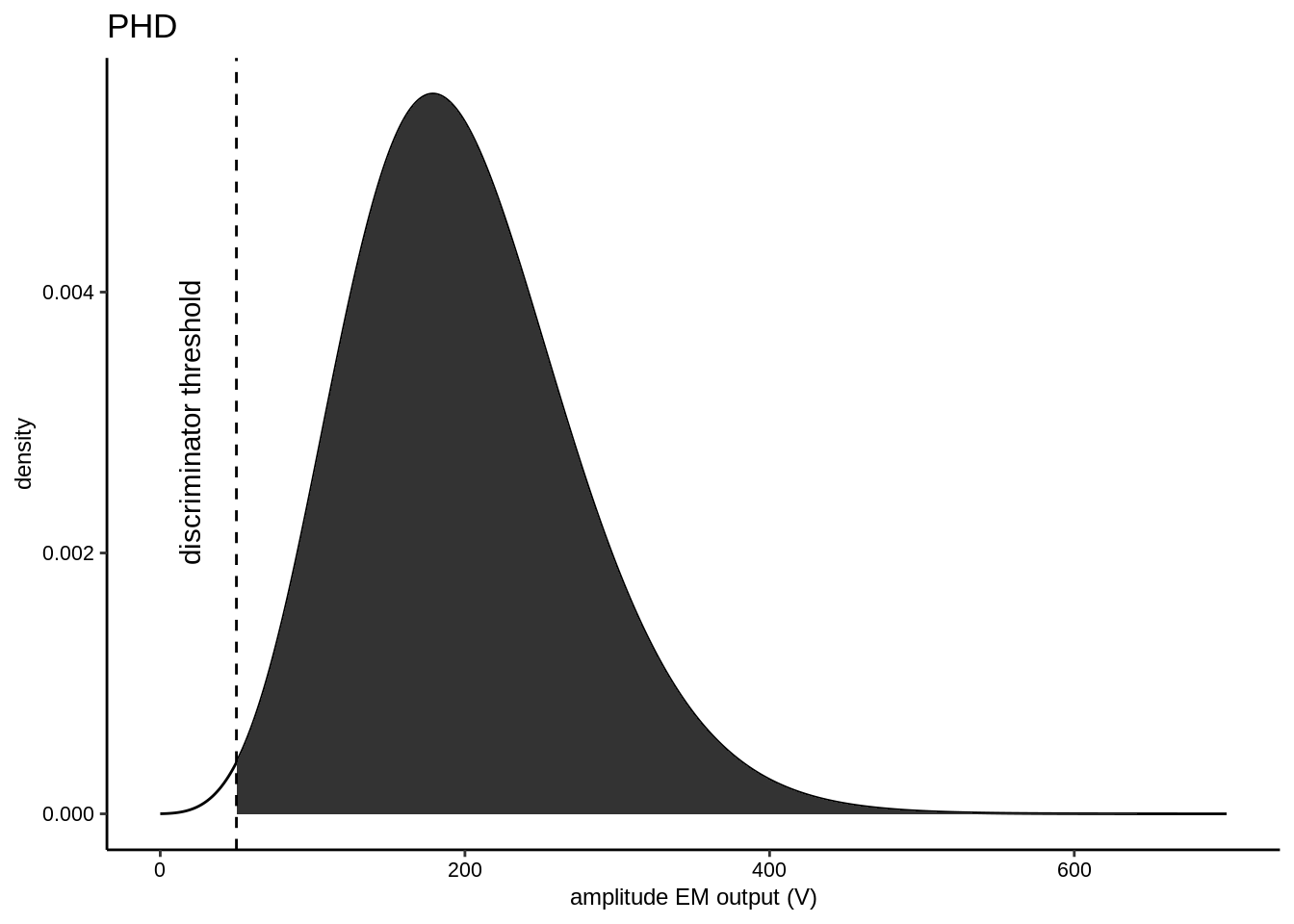
An example of a typical PHD distribution. The effect of the discriminator threshold on the EM Yield is examplified by the shaded area underneath the probability density function, which would pertain to the probability of an EM output to be larger than the threshold

Figure 1.2: An example of a typical PHD distribution. The effect of the discriminator threshold on the EM Yield is examplified by the shaded area underneath the probability density function, which would pertain to the probability of an EM output to be larger than the threshold

This causes the true EM Yield $Y_{EM}$ to be smaller than 100% (see Fig. 1.2). The PHD distribution adheres to the following principles:

Poisson statistics can account for the random processes involved in the initial generation of secondary ions (coupled to incident ions at the first dynode) and for each stage of successive multiplication by secondary electron generation at subsequent dynodes along the EM channel.
A geometric distribution describes the success of amplification at each dynode, which is independent and with identical probabilities at each dynode.
Successive stages of electron amplification results in a compounding of these random processes, but the shape of the PHD converges after the fourth or fifth stage of amplification (Dietz and Hanrahan 1978).

Given the previous points, the probability of the whole amplification process can be gauged by taking a geometric compounded Poisson (or Polya-Aeppli) random variable (Dietz 1970; Dietz and Hanrahan 1978), which can be described by the following equation:

\[\begin{equation} P(x;\lambda, p) \; = \; \text{Pr}(X = x) \; =\\ \begin{cases} e^{-\lambda}, & \text{if } x = 0 \\ e^{-\lambda}\sum_{n=1}^{y}{\frac{\lambda^n}{n!}}\binom{y-1}{n-1}p^{\lambda-n}(1-p)^n, & \text{if } x = 1,2,... \\ \end{cases} \tag{1.1} \end{equation}\]

where $\lambda$ and $p$ determine, respectively, the location and the shape of the Polya-Aeppli probability distribution, see Burden (2014) for a full derivation of this equation and the associated parameters. Note, that the discriminator threshold causes $x > 0$. Furthermore, if $p$ = 0, the Polya-Aeppli probability distribution simplifies to a Poisson distribution.

The discriminator threshold value, the mean and variance of the measured PHD, can be used to calculate the probability that of successful ion-to-electron conversions before the analysis. This provides a means to get an accurate estimate of the true EM Yield ($Y_{EM}$).

Th function cor_yield calculates the yield with a given mean (mean_PHD), standard deviation (SD_PHD), and threshold value for the PHD, and makes use of the package pPolyaAeppli (Burden 2014).

The $Y_{EM}$ can then be used to calculate the corrected counts and count rates.

\[\begin{equation} X_{i}^* = \frac{X_i }{Y_{EM}} \tag{1.2} \end{equation}\]

# original count rate of a chemical species
x <- 30000
# function to correct count rate based on EM Yield
cor_yield(x, mean_PHD = 210, SD_PHD = 60, thr_PHD = 50)
#> [1] 30007.95

The shape of the PHD distribution changes with the age of the EM but its deleterious effect on secondary ion-to-electron conversion can be alleviated by changing the EMHV. Tools for the assessment of EM deterioration is dealt with in a subsequent section.

1.2.1.2 Dead time

Another bias introduced by EM ion detection devices is the time associated for recovery after an ion hits the first dynode. During the intermediate time, a second ion arriving at the same time can then not be recorded because of the electronic paralysis of the EM. Although this dead time ($t_{ns}$) is small ($44\,$ns), high count frequencies can cause the cumulate effect of this re-occurring phenomenon to become significant for the final count numbers. The count rates can be corrected by the following equation:

\[\begin{equation} X_{i}^{*} = \frac{X_i}{1- X_i \times t_{ns} \times 10^9} \tag{1.3} \end{equation}\]

The function cor_DT is implemented to correct for this systematic bias of EM devices.

# corrected count rate for a deadtime of 44 ns
cor_DT(x, 44)
#> [1] 30039.65

For a convenient workflow the functions that correct for EM count biases are wrapped in the function cor_IC(). This function takes the tibble as loaded with the function read_IC() (see vignette IC-read) and requires setting the following arguments: N, a variable for the raw ion count;t, a variable for the time increments; Det a character string or variable identifying the ion detection system: EM ("EM") or FC ("FC"); deadtime, a numeric value for the deadtime in nanoseconds; and thr_PHD, a numeric value for the discriminator threshold.

# Use point_example() to access the examples bundled with this package 

# Carry-out the routine point workflow 

# Carry-out the routine point workflow
# Raw data containing 13C and 12C counts on carbonate
tb_rw <- read_IC(point_example("2018-01-19-GLENDON"), meta = TRUE)

# processing raw ion count data
tb_pr <- cor_IC(tb_rw)

The function returns the original tibble but adds the variables: Xt.rw, ion count rates uncorrected for detection device-specific biases; Xt.pr, ion count rates corrected for detection device-specific biases; and N.pr, counts corrected for detection device-specific biases.

1.2.2 Analytical bias introduced by Faraday Cups

To be included in the future.

1.3 Systematic bias by ionization yield fluctuations

In contrast to EM yield, ionization yield defines the efficiency whereby secondary ions are generated per incident primary ion. The probability whereby the primary beam produced secondary ions depends strongly on properties of the substrate (matrix effects) and the evolving sputter pit as well as the machine settings, such as the beam type (Cs⁺ and O^-) and sample charging. The latter effect of sample charge build-up combined with the deepening of the sputter pit are connected to large systematic biases seen in the count rates of individual ions (see Fig. 1.3) throughout a single analysis (Fitzsimons, Harte, and Clark 2000).

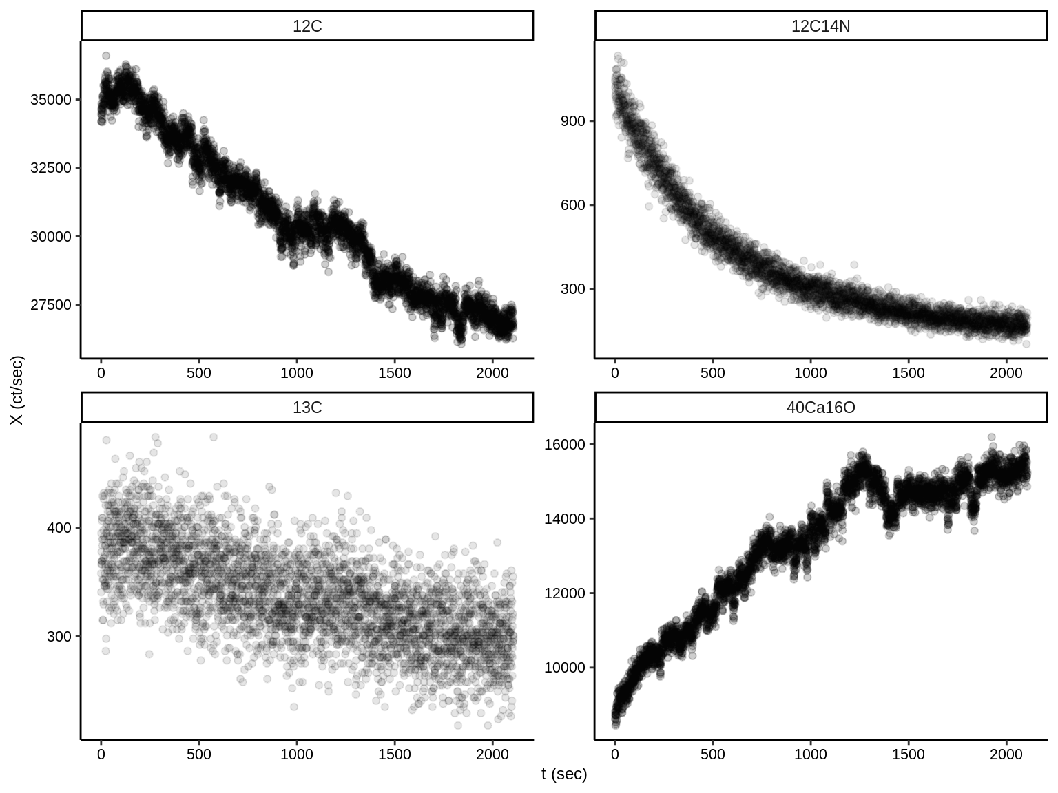
Changes in the ionization potential examplified by single ion monotonic trends in count rates over subsequent measurements of a single analysis with the NanoSIMS Cameca50L.

Figure 1.3: Changes in the ionization potential examplified by single ion monotonic trends in count rates over subsequent measurements of a single analysis with the NanoSIMS Cameca50L.

The systematic changes induced by ionization differences in count rate affect modulate count rates for both isotopes of the same equally (see Fig. 1.3). From the the formula for exact propagation of error (Ku 1966) it can further be deduced that the error of co-variate ratios, such as for isotope ratios ($R$), will effectively be dampened by the co-variate term in the equation (see vignette IC-precision) and Fitzsimons, Harte, and Clark (2000). However, this is not the case for none-isotope ion ratios and so their propagated error is also largely an effect of this systematic variance induced by ionization trends (see Fig. 1.4).

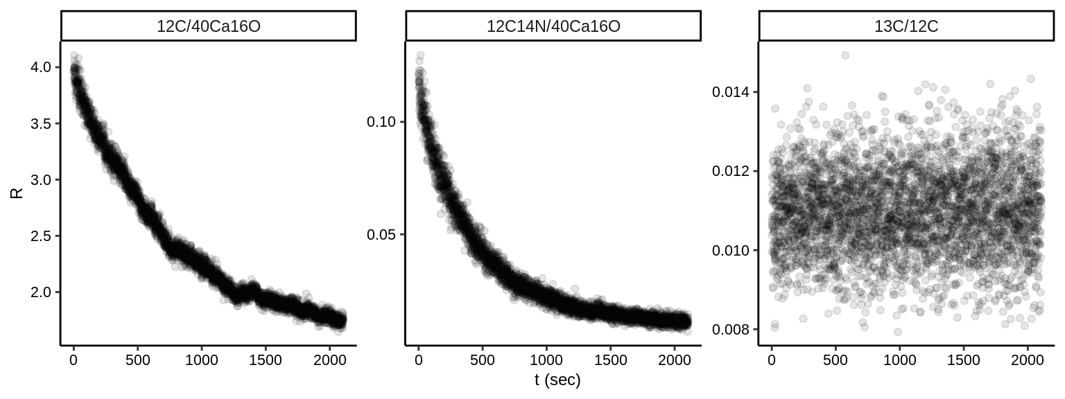
Figure 1.4: Changes in the ratios of none-isotope and isotope ratios compared.

Upon plotting the count rate ratios against time (Fig. 1.4), it becomes apparent that the none-isotope ratios are affected by monotonic trends over the duration of the analysis. This effect reflects the differential ionization potentials and trajectories of secondary beam stabilization over the analysis (as explained above; Fig. 1.3).

\[\begin{equation} y_t = l_0 + T_t + P_t + \epsilon_t \tag{1.4} \end{equation}\]

Time-series can be decomposed in several components (Eq. (1.4)); the base level or mean of the time series; $l0$, a structural trend component $T_t$ which change dependent on the time increment, a cyclical component $P_t$ and a noise component $\epsilon_t$. Structural trends of a variable (i.e. count rates of species $X_i^a$) based on the independent variable time (i.e. $n$- series of measurements) can be described with regression analysis with the simplest implementation presented by the linear regression model:

\[\begin{equation} \hat{y}_t = \beta_0 + \beta_1x_t + \epsilon_t \tag{1.5} \end{equation}\]

The General Additive Model (GAM) is an extension of this model with addition of a smoothing function replacing the linear term of the previous function (Eq (1.5):

\[\begin{equation} \hat{y}_t = \beta_0 + f(x_1) + \epsilon_t \tag{1.6} \end{equation}\]

The function predict_ionize() provides a convenient implementation of GAM from the package mgcv, which has the function s(), to define the smooth function in the gam() call. The protocol implemented assures effective bandwidth selection based on goodness of fit measured with a penalized information criterion. With the knowledge that ionization is represented as global trend, this allows for subtraction of the model fit from the actual count rate data to allow for a more accurate assessment of the $l0$ as well as the random component $\epsilon_t$ informing about the precision unbiased by a large systematic offset.

\[\begin{equation} X_i^a* = \bar{\hat{X}}^a + (X_i^a - \hat{X}_i^a) \tag{1.7} \end{equation}\]

The point package provides additional diagnostic tools to assess whether the model represents an under- or over-fit on the data (see vignette IC-diagnostics).

tb_dt <- predict_ionize(tb_pr, file.nm)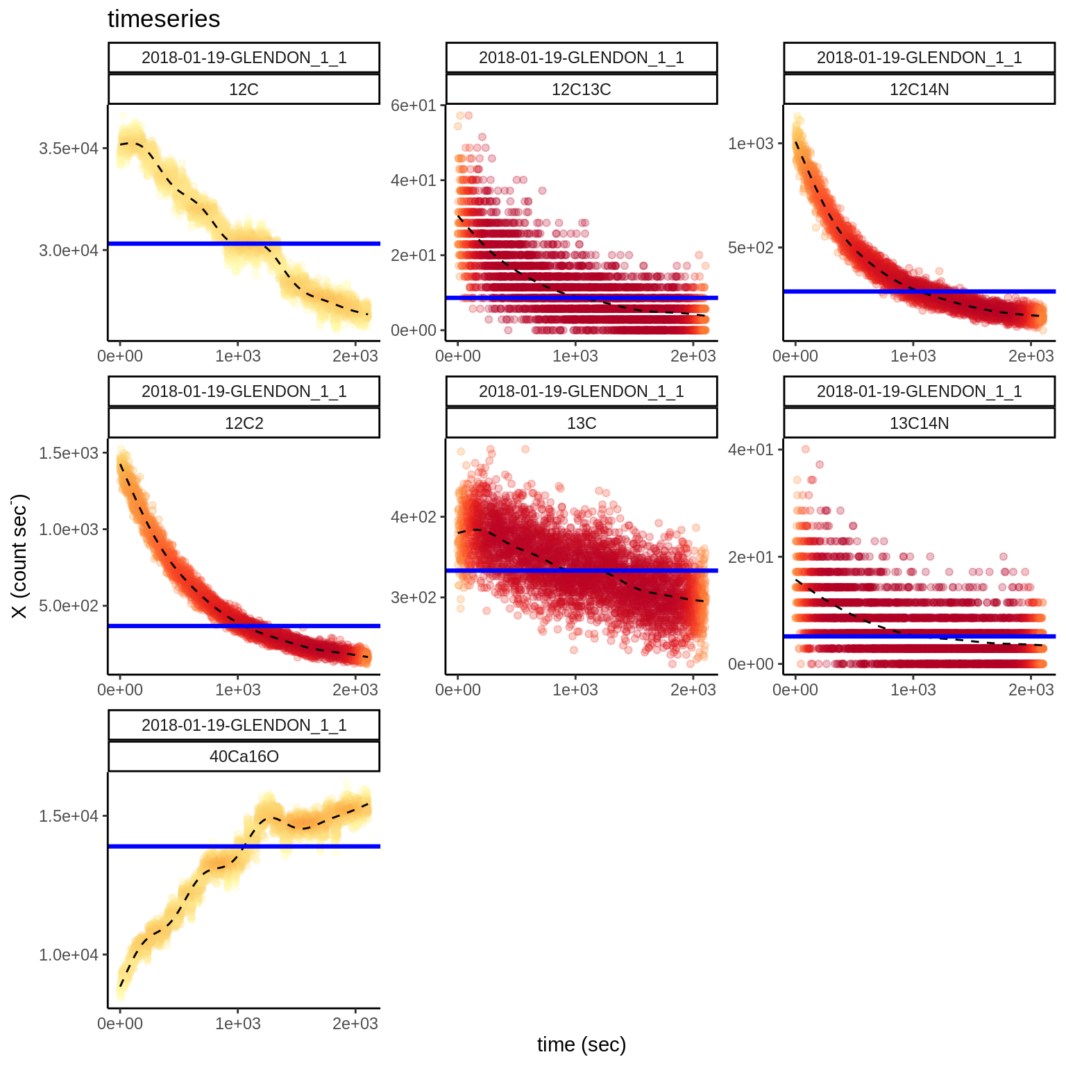

Figure 1.5: GAM predicted model fit (dashed black line) to single ion count rates and median count rate (solid blue line).

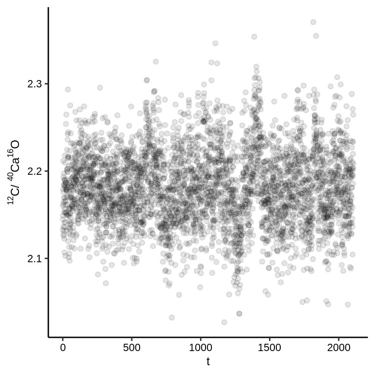
$An extraction of the $l0$ and $\epsilon_t$ components, by appliciation of Eq. \@ref(eq:detr), and thereby yielding corrected none-isotope ion count ratios.$

Figure 1.6: An extraction of the $l0$ and $\epsilon_t$ components, by appliciation of Eq. (1.7), and thereby yielding corrected none-isotope ion count ratios.

References

Burden, Conrad J. 2014. “An R Implementation of the Polya-Aeppli Distribution.” http://arxiv.org/abs/1406.2780.

Dietz, L. A. 1970. “General method for computing the statistics of charge amplification in particle and photon detectors used for pulse counting.” International Journal of Mass Spectrometry and Ion Physics 5 (1-2): 11–19. https://doi.org/10.1016/0020-7381(70)87002-4.

Dietz, L. A., and L. R. Hanrahan. 1978. “Electron multiplier-scintillator detector for pulse counting positive or negative ions.” Review of Scientific Instruments 49 (9): 1250–6. https://doi.org/10.1063/1.1135590.

Fitzsimons, I. C. W., B. Harte, and R. M. Clark. 2000. “SIMS stable isotope measurement: counting statistics and analytical precision.” Mineralogical Magazine 64 (01): 59–83. https://doi.org/10.1180/002646100549139.

Ku, H. H. 1966. “Notes on the use of propagation of error formulas.” Journal of Research of the National Bureau of Standards, Section C: Engineering and Instrumentation 70C (4): 263. https://doi.org/10.6028/jres.070c.025.

Slodzian, Georges, M Chaintreau, R Dennebouy, and A Rousse. 2001. “Precise in situ measurements of isotopic abundances with pulse.” The European Physical Journal Applied Physics 14: 199–231. https://doi.org/10.1051/epjap:2001160.

Martin Schobben