3. Patterns and models
model.Rmd
library(PAGES)The datasauRus and tidyverse packages
This exercise is largely constructed around the datasauRus (Locke and D’Agostino McGowan 2018) package. In addition, I will use again the tidyverse collection packages ggplot2 (Wickham et al. 2020; Wickham 2016) for plotting and dplyr (Wickham et al. 2021) for data manipulations.
Data
The datasaurus_dozen dataset of the datasauRus (Locke and D’Agostino McGowan 2018) package consists of one categorical variable dataset representing subsets of the data, which, in turn, all contain an x and y variable.
Model datasauRus
First, we will model all datasets with a conventional least square linear regression with geom_smooth() and by setting the argument method to "lm". We see then that all subsets can be fitted with more-or-less similar models.
ggplot(data = datasaurus_dozen) +
  geom_smooth(mapping = aes(x = x, y = y, colour = dataset), method = "lm") +
  theme_classic() +
  theme(legend.position = "none") +
  facet_wrap(facets = vars(dataset), ncol = 3)
#> `geom_smooth()` using formula 'y ~ x'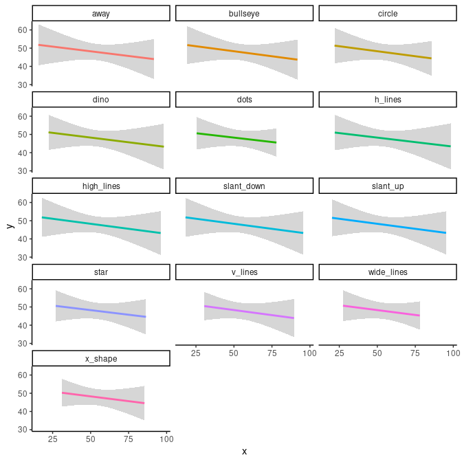
The theme() and theme_classic() functions in this construction dictate certain visual aspects of the plots. They are of no further relevance.
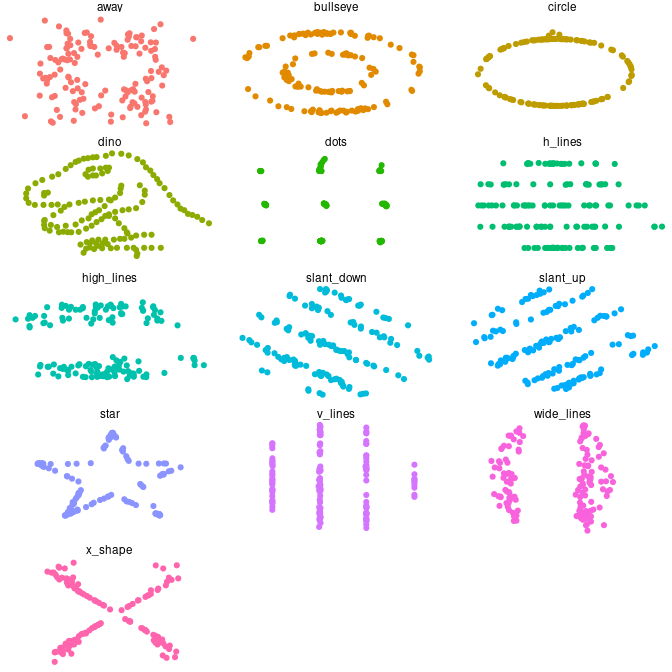
Visualize datasauRus
These plots are a variant of plots known as Anscombe plots, after the statistician Francis Anscombe, demonstrating the importance of graphing data before analysing it.
ggplot(data = datasaurus_dozen) +
  geom_point(mapping = aes(x = x, y = y, colour = dataset)) +
  theme_void() +
  theme(legend.position = "none") +
  facet_wrap(facets = vars(dataset), ncol = 3)